Import packages
Load sample dataset
##   start stop event        age      year surgery transplant id
## 1     0   50     1 -17.155373 0.1232033       0          0  1
## 2     0    6     1   3.835729 0.2546201       0          0  2
## 3     0    1     0   6.297057 0.2655715       0          0  3
## 4     1   16     1   6.297057 0.2655715       0          1  3
## 5     0   36     0  -7.737166 0.4900753       0          0  4
## 6    36   39     1  -7.737166 0.4900753       0          1  4
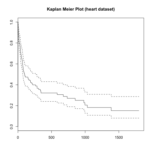
Performing survival analysis with heart dataset
survival <- Surv(heart$start, heart$stop, heart$event == 1) # creating survival object
surv_fit <- survfit(survival ~ 1) # fit a survival curve
plot(surv_fit, main = "Kaplan Meier Plot (heart dataset)")
## $n
## [1] 172
##
## $time
##  [1]    1    2    3    5    6    8    9   12   16   17   18   21   28   30
## [15]   32   35   36   37   39   40   43   45   50   51   53   58   61   66
## [29]   68   69   72   77   78   80   81   85   90   96  100  102  110  149
## [43]  153  165  186  188  207  219  263  285  308  334  340  343  584  675
## [57]  733  852  980  996 1032 1387
##
## $n.risk
##  [1] 103 102  99  96  94  92  91  89  88  85  84  83  81  80  78  77  76
## [18]  75  74  72  70  69  68  67  66  65  64  63  62  60  59  57  56  55
## [35]  54  53  52  51  50  49  47  45  44  43  41  40  39  38  37  35  33
## [52]  32  31  29  21  17  16  14  11  10   9   6
##
## $n.event
##  [1] 1 3 3 2 2 1 1 1 3 1 1 2 1 1 1 1 1 1 1 2 1 1 1 1 1 1 1 1 2 1 2 1 1 1 1
## [36] 1 1 1 1 1 1 1 1 1 1 1 1 1 1 2 1 1 1 1 1 1 1 1 1 1 1 1
##
## $n.censor
##  [1] 2 3 3 5 1 2 0 6 2 2 1 5 8 0 5 1 2 2 2 0 2 0 2 2 0 2 1 0 2 0 1 0 1 0 0
## [36] 2 0 1 0 0 1 2 0 1 1 0 0 1 0 1 0 1 1 0 7 3 0 1 2 0 0 2
##
## $n.enter
##  [1] 105   3   3   5   1   2   0   5   2   2   1   5   8   0   4   1   2
## [18]   2   1   0   2   0   2   2   0   2   1   0   2   0   1   0   1   0
## [35]   0   2   0   1   0   0   0   1   0   1   0   0   0   1   0   0   0
## [52]   1   0   0   0   0   0   0   0   0   0   0
Perform survival analysis against heart surgery status
heart$surgery <- as.factor(heart$surgery)
surv_fit2 <- survfit(survival ~ heart$surgery) # fit a survival curve
plot(surv_fit2, main="Kaplan Meier Plot by Surgery", xlab="Time in Days", ylab="Survival Proportion", col=c(1:2))
legend('topright', c("Surgery: No","Surgery: Yes"), lty=1, col=c(1:2))
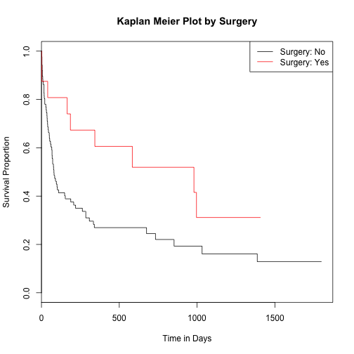
Assess significance of survival by surgery status
survdiff(Surv(time = heart$start, event = heart$event == 1) ~ heart$surgery)
## Call:
## survdiff(formula = Surv(time = heart$start, event = heart$event ==
##     1) ~ heart$surgery)
##
##                   N Observed Expected (O-E)^2/E (O-E)^2/V
## heart$surgery=0 143       66     58.7     0.902      4.56
## heart$surgery=1  29        9     16.3     3.255      4.56
##
##  Chisq= 4.6  on 1 degrees of freedom, p= 0.0328
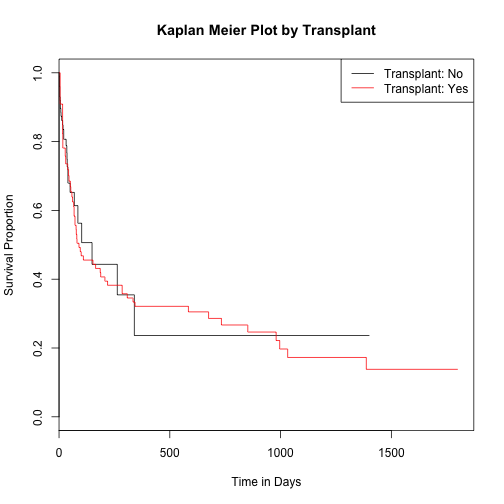
Survival analysis by transplant status
heart$transplant <- as.factor(heart$transplant)
surv_fit3 <- survfit(survival ~ heart$transplant)
plot(surv_fit3, main="Kaplan Meier Plot by Transplant", xlab="Time in Days", ylab="Survival Proportion", col=c(1:2))
legend('topright', c("Transplant: No","Transplant: Yes"), lty=1, col=c(1:2))
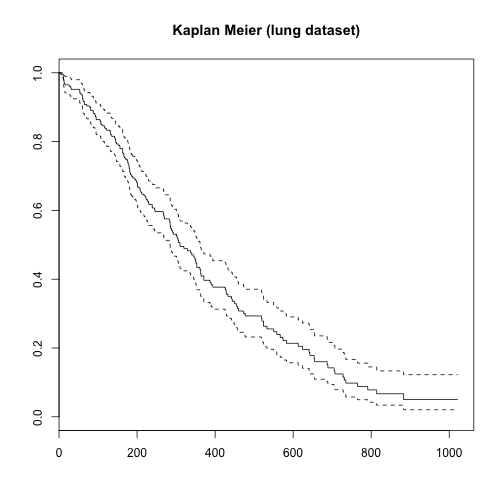
Performing survival analysis with lung dataset
survival_lung <- Surv(time = lung$time, event = lung$status == 2, type='right')
surv_fit3 <- survfit(survival_lung ~ 1)
plot(surv_fit3, main = "Kaplan Meier (lung dataset)")
Survival analysis by sex
lung$sex <- as.factor(lung$sex)
surv_fit4 <- survfit(survival_lung ~ lung$sex)
plot(surv_fit4, main="Kaplan Meier Plot by Sex", xlab="Time in Days", ylab="Survival Proportion", col=c(1:2))
legend('topright', c("Male","Female"), lty=1, col=c(1:2))
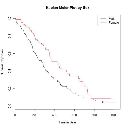
Assess significance of survival by sex
survdiff(Surv(time = lung$time, event = lung$status == 2) ~ lung$sex)
## Call:
## survdiff(formula = Surv(time = lung$time, event = lung$status ==
##     2) ~ lung$sex)
##
##              N Observed Expected (O-E)^2/E (O-E)^2/V
## lung$sex=1 138      112     91.6      4.55      10.3
## lung$sex=2  90       53     73.4      5.68      10.3
##
##  Chisq= 10.3  on 1 degrees of freedom, p= 0.00131
Survival analysis by ECOG performance score
lung$ph.ecog <- as.factor(lung$ph.ecog) #ECOG performance score (0=good 5=dead)
surv_fit4 <- survfit(survival_lung ~ lung$ph.ecog)
plot(surv_fit4, main="Kaplan Meier Plot by ECOG Performance", xlab="Time in Days", ylab="Survival Proportion", col=c(1:5))
legend('topright', c("Ecog=0","Ecog=1", "Ecog=2", "Ecog=3"), lty=1, col=c(1:5))
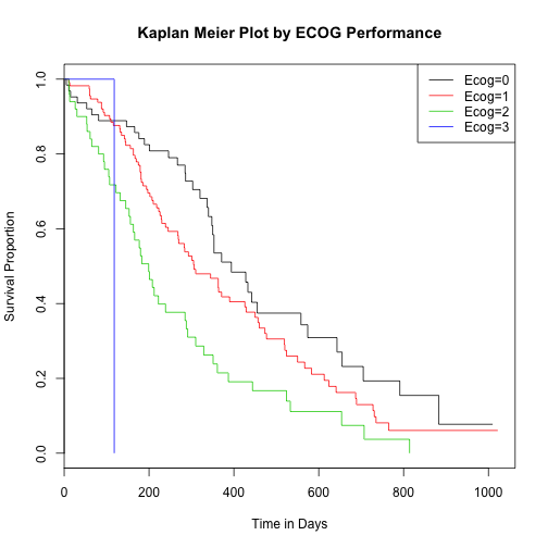
Assess significance of survival by ECOG
survdiff(Surv(time = lung$time, event = lung$status == 2) ~ lung$ph.ecog)
## Call:
## survdiff(formula = Surv(time = lung$time, event = lung$status ==
##     2) ~ lung$ph.ecog)
##
## n=227, 1 observation deleted due to missingness.
##
##                  N Observed Expected (O-E)^2/E (O-E)^2/V
## lung$ph.ecog=0  63       37   54.153    5.4331    8.2119
## lung$ph.ecog=1 113       82   83.528    0.0279    0.0573
## lung$ph.ecog=2  50       44   26.147   12.1893   14.6491
## lung$ph.ecog=3   1        1    0.172    3.9733    4.0040
##
##  Chisq= 22  on 3 degrees of freedom, p= 6.64e-05