Following post shows an overview of Principle Components Analysis (PCA) using the Chronic Kidney Disease dataset, from UCI Machine Learning Repository. PCA is a dimensionality reduction technique that converts correlated predictors into a set of uncorrelated predictors called principle components using orthogonal transformations.
Chronic Kidney Disease Data, collected from a hospital for nearly 2 months, contains features that can be used to predict chronic kidney disease incidence. Collected attributes include age, blood pressure, specific gravity, albumin, sugar, red blood cells, pus cell, pus cell clumps, bacteria, blood glucose random, blood urea, serum creatinine, sodium, potassium, hemoglobin, packed cell volume, white blood cell count, red blood cell count, hypertension, diabetes mellitus, coronary artery disease, appetite, pedal edema and anemia. Features are used to predict coronary kidney disease incidence as defined by the class predictor. For further details about feature definition and data collection, see citation.
Import packages
library(stats)
library(rpart)
Read the Chronic Kidney Disease dataset (archived) from UCI Machine Learning Repository
ckd_data <- read.csv("https://raw.githubusercontent.com/ajav17/Chronic-Kidney-Disease-UCI-Dataset/master/chronic_kidney_disease_dataset.csv")
ckd_data <- ckd_data[ ,!(colnames(ckd_data) %in% c("rbc", "pc"))]
Replace missing values with NA for later imputation
ckd_data[ckd_data == "?"] <- NA
ckd_data <- base::droplevels(ckd_data)
Convert variable types
ckd_data$age <- as.numeric(as.character(ckd_data$age))
ckd_data$bp <- as.numeric(as.character(ckd_data$bp))
ckd_data$sg <- as.numeric(as.character(ckd_data$sg))
ckd_data$al <- as.numeric(as.character(ckd_data$al))
ckd_data$su <- as.numeric(as.character(ckd_data$su))
ckd_data$bgr <- as.numeric(as.character(ckd_data$bgr))
ckd_data$bu <- as.numeric(as.character(ckd_data$bu))
ckd_data$sc <- as.numeric(as.character(ckd_data$sc))
ckd_data$sod <- as.numeric(as.character(ckd_data$sod))
ckd_data$pot <- as.numeric(as.character(ckd_data$pot))
ckd_data$hemo <- as.numeric(as.character(ckd_data$hemo))
ckd_data$pcv <- as.numeric(as.character(ckd_data$pcv))
ckd_data$wbcc <- as.numeric(as.character(ckd_data$wbcc))
ckd_data$rbcc <- as.numeric(as.character(ckd_data$rbcc))
ckd_data$pcc <- as.factor(ckd_data$pcc)
ckd_data$ba <- as.factor(ckd_data$ba)
ckd_data$htn <- as.factor(ckd_data$htn)
ckd_data$dm <- as.factor(ckd_data$dm)
ckd_data$cad <- as.factor(ckd_data$cad)
ckd_data$appet <- as.factor(ckd_data$appet)
ckd_data$pe <- as.factor(ckd_data$pe)
ckd_data$ane <- as.factor(ckd_data$ane)
ckd_data$class <- as.factor(ckd_data$class)
Impute missing values with mean
ckd_copy <- ckd_data
imputeMean <- function(x)
    {
        if (class(x) == "numeric")
        {
            replace(x, is.na(x), mean(x, na.rm = TRUE))
        }
    }

ckd_data <- lapply(ckd_data, imputeMean)
ckd <- data.frame(t(do.call(rbind, ckd_data)))

ckd <- cbind(ckd, ckd_copy$pcc, ckd_copy$ba, ckd_copy$htn,
           ckd_copy$dm, ckd_copy$cad, ckd_copy$appet, ckd_copy$pe, ckd_copy$ane, ckd_copy$class)
colnames(ckd) <- c("age", "bp", "sg", "al", "su", "bgr", "bu", "sc", "sod", "pot", "hemo", "pcv", "wbcc", "rbcc",
                "pcc", "ba", "htn", "dm", "cad", "appet", "pe", "ane", "class")
Omit any remaining values
ckd_data <- stats::na.omit(ckd)
nrow(ckd_data)
PCA
Selecting numeric predictors for PCA
numeric <- sapply(ckd_data, is.numeric)
ckd_data_num <- ckd_data[, numeric]
Partitioning train and test sets
n = nrow(ckd_data)
index = base::sample(1:n, size = round(0.75*n), replace = FALSE)
train2 = ckd_data[index ,]
test2 = ckd_data[-index ,]

num_index_test <- sapply(test2, is.numeric)
num_index_train <- sapply(train2, is.numeric)
train2_num <- train2[, num_index_train]
test2_num <- test2[, num_index_test]
Applying principle components
principle_comp <- prcomp(train2_num, center = TRUE, scale. = T)
dim(principle_comp$x)
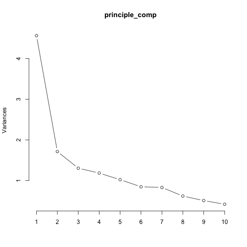
## Standard deviations (1, .., p=14):
##  [1] 2.1356539 1.3095935 1.1427020 1.0895520 1.0118050 0.9217633 0.9126997
##  [8] 0.7884078 0.7144548 0.6482579 0.5699756 0.5500808 0.4665634 0.3566861
##
## Rotation (n x k) = (14 x 14):
##              PC1         PC2         PC3         PC4          PC5
## age   0.18568534 -0.17753082 -0.01522342  0.07163808 -0.259122149
## bp    0.14224600 -0.06096325  0.01023196 -0.21816811 -0.753714791
## sg   -0.28408381  0.19397838 -0.08372604 -0.09834507 -0.079331169
## al    0.32074464 -0.09668204  0.11527488 -0.02914664  0.304899748
## su    0.18225833 -0.47366373 -0.45419059  0.02005034 -0.030996731
## bgr   0.20315545 -0.48387235 -0.31621651  0.21516216 -0.003578622
## bu    0.32176736  0.27937508 -0.15752930 -0.22991428  0.190878611
## sc    0.24473474  0.40660766 -0.35624425  0.27295528  0.041297545
## sod  -0.22178142 -0.32830865  0.18627870 -0.58252764  0.070832354
## pot   0.12879353  0.07563276 -0.42480054 -0.61217479  0.241389043
## hemo -0.39747992 -0.04151640 -0.28043678  0.08301244  0.027836462
## pcv  -0.39742088 -0.03274801 -0.26889647  0.09283823  0.067927108
## wbcc  0.05639762 -0.30642626  0.32113766  0.16222212  0.389218295
## rbcc -0.37268972 -0.07563917 -0.22830468  0.08224969  0.078949133
##              PC6          PC7          PC8         PC9         PC10
## age   0.38107638 -0.836458433  0.034051016 -0.10113476  0.030437335
## bp    0.28768385  0.416439791 -0.070003826 -0.26565074  0.044451928
## sg    0.28809467  0.049686527  0.823316652  0.28234625  0.105209625
## al   -0.05405720  0.083316805  0.377341403 -0.70660250  0.312758271
## su    0.01215736  0.167991350  0.107505491  0.11614701 -0.219389115
## bgr  -0.23253742  0.033653576  0.186836060  0.16397884  0.059675977
## bu    0.07736250 -0.043518758  0.160869073 -0.14260331 -0.606381283
## sc    0.26438650  0.091288016 -0.128929647 -0.02475725 -0.157213404
## sod  -0.02494634 -0.085140048  0.005944041 -0.06364227 -0.380939539
## pot   0.16013606 -0.037867603 -0.236084281  0.16044111  0.474656659
## hemo  0.12030748 -0.048457282 -0.086920409 -0.22563429  0.118676716
## pcv   0.07908303 -0.005326901 -0.060800312 -0.31590475  0.023707811
## wbcc  0.70375227  0.256511416 -0.123270476  0.15166872 -0.008497769
## rbcc  0.11717638  0.032654766 -0.050176955 -0.27452758 -0.242840195
##              PC11        PC12        PC13          PC14
## age   0.002140315  0.05017720 -0.01258517  0.0402359275
## bp   -0.140660707 -0.07834737 -0.02658567  0.0002937661
## sg   -0.000282000  0.02889846  0.05813752  0.0192951310
## al    0.089281175  0.10591501  0.10242703 -0.0404737905
## su    0.579438952  0.23498919 -0.20477001  0.0180125332
## bgr  -0.562197308 -0.29468777  0.23353223 -0.0169339759
## bu   -0.201342020 -0.31309454 -0.37423449 -0.0624076547
## sc    0.115437689  0.05904818  0.65927189 -0.0041900558
## sod   0.083534380 -0.06632398  0.54310495 -0.0236515783
## pot  -0.133772009  0.08409883 -0.05540173  0.0481587674
## hemo  0.145279970 -0.37742270 -0.04932235 -0.7061277301
## pcv   0.088802381 -0.38335927 -0.04611510  0.6986644563
## wbcc -0.079468220 -0.11017304 -0.06431116  0.0077562753
## rbcc -0.454289249  0.65014871 -0.08588973 -0.0464742259
## Importance of components:
##                           PC1    PC2     PC3     PC4     PC5     PC6
## Standard deviation     2.1357 1.3096 1.14270 1.08955 1.01180 0.92176
## Proportion of Variance 0.3258 0.1225 0.09327 0.08479 0.07312 0.06069
## Cumulative Proportion  0.3258 0.4483 0.54156 0.62635 0.69948 0.76017
##                           PC7    PC8     PC9    PC10    PC11    PC12
## Standard deviation     0.9127 0.7884 0.71445 0.64826 0.56998 0.55008
## Proportion of Variance 0.0595 0.0444 0.03646 0.03002 0.02321 0.02161
## Cumulative Proportion  0.8197 0.8641 0.90053 0.93055 0.95375 0.97536
##                           PC13    PC14
## Standard deviation     0.46656 0.35669
## Proportion of Variance 0.01555 0.00909
## Cumulative Proportion  0.99091 1.00000
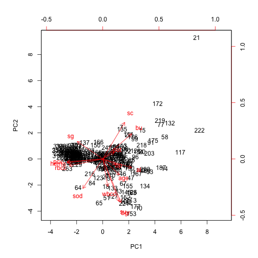
Biplot
biplot(principle_comp, scale = 0)
Scree plot
plot(principle_comp, type = "l")
Training data with appropriate components
train_prin <- data.frame(train2$class, principle_comp$x)
train_prin <- train_prin[, 1:10] # select 9 components
Model decision tree
tree_prin <- rpart(train2.class ~ ., data = train_prin)
Construct test data from PCA
# Converting test to PCA
test_prin <- as.data.frame(predict(principle_comp, test2_num))
Predict decision tree on test data
# Select 9 components and predict on test set
test_prin <- test_prin[, 1:9]
tree_predict <- predict(tree_prin, test_prin, type = "class")
Calculating accuracy
tab <- base::table(tree_predict, test2$class)
round(sum(diag(tab))/sum(tab), 3)